15-418 Final Project

Parallellized Sequential Pattern Mining

Anna Tan

Proposal | Checkpoint | Final Report

Summary

We parallellized two common data mining algorithms for sequential pattern mining on multi-core CPU platforms, PrefixSpan and the GSP algorithm. We evaluated the performance between the sequential implementations and the parallel implementations across three different datasets. Our 16 thread implementation for the GSP algorithm achieved up to 7.1x speedup, whereas our 16 thread implementation for the PrefixSpan algorithm achieved up to 4.9x speedup.

Background

Sequential pattern mining is used to discover statistically relevant patterns in large data sets where the data is assumed to be delivered in sequence. It is used in a wide variety of applications, including consumer behavior discovery, DNA pattern discovery, and natural language categorization.

A sequence in a sequence database is an ordered list of items. It would look something like <a, b, d, d, b>. A sequential pattern is any (possibly non-contiguous) subsequence of the sequence. In this sequence, a sequential pattern can be <a>, <a, d>, or <b, d, b>. A sequential pattern mining algorithm takes as input a sequence database and a minimum support threshold (minsup) in percentage, to output all frequent sequential patterns with at least minsup of the database having the pattern.

For example, say our sequence database contains the following four sequences: s1 = <a, b, d, d, b>, s2 = <b, c, b, a>, s3 = <d, d, b>, s4 = <a, b, d, a>, and minsup is 0.5. The frequent sequential patterns in this database are <a>, <b>, <d>, <a, b>, <a, d>, <b, d>, <d, d>, <a, b, d>, and <d, d, b>.

Two popular algorithms for finding frequent sequential patterns are PrefixSpan and the GSP (Generalized Sequential Pattern) algorithm.

PrefixSpan

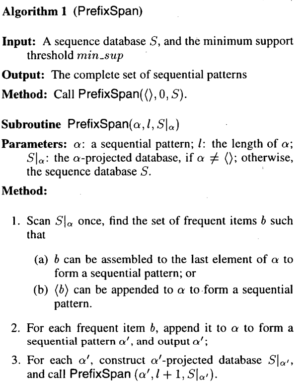
PrefixSpan (Pei et al.) finds these sequential patterns by finding the frequent items in the database (via support counting), and for each of these items, generate a projected database, and recursively call the subroutine with the projected database.

The size of the projected database decreases as we continue to project, due to the fact that the number of supports cannot increase going from, say, <a, b> to <a, b, d>.

In the example above, we would have <a>, <b>, <d> as our initial frequent items. For <a>, we would gnerate a projected database that looks like s1' = <b, d, d, b>, s4' = <b, d, a>. From the projection, our frequent items are now b and d. So for the frequent sequential pattern <a, d>, we would generate a projected database that looks like s1'' = <d, b>, s4'' = <a>.

GSP Algorithm

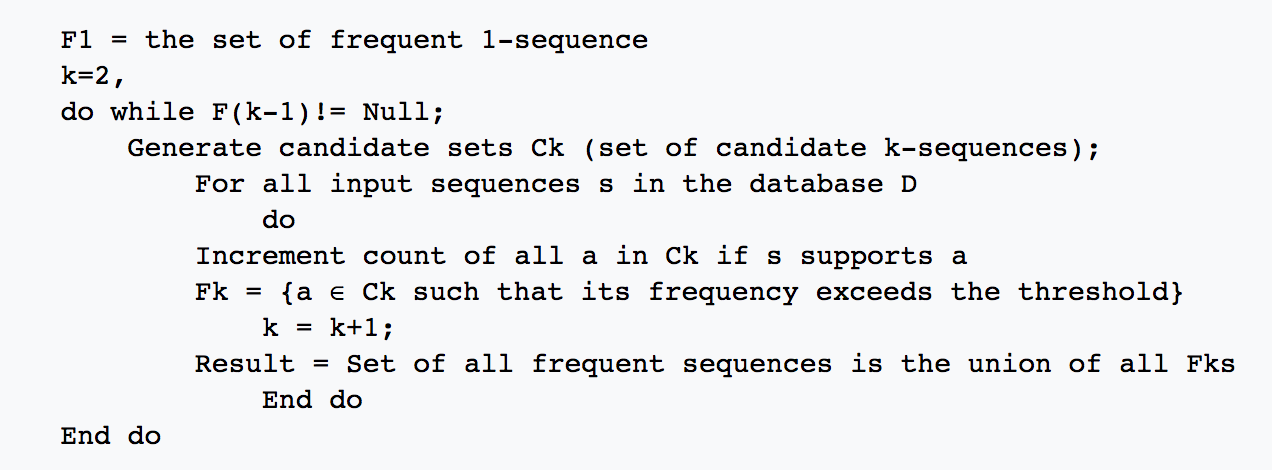
The GSP algorithm (Srikant & Agrawal), on the other hand, generates all possible k-sequences from frequent k-1 sequences by "joining" any two sequences in a process called candidate generation, and then checks how much support each of these candidates has to get the frequent candidates. It then repeats to generate all possible k+1-sequences, etc.

In the example above, we would have <a>, <b>, <d> as our initial frequent 1-sequences. We then join any two of the sequences to create candidates, giving us <a, a>, <a, b>, <a, d>, <b, a>, <b, b>, <b, d>, <d, a>, <d, b>, <d, d>. Then, we count, for each of these candidates, the number of supports they get from the database, and retrieve the frequent 2-sequences <a, b>, <a, d>, <b, d>, <d, d>.

In both of these algorithms, we represent items as unsigned integers and sequences as a vector of items. Support counting uses a map from the sequences to a integer count, which increments for every support. We also use set to ensure we don't overcount by keeping track of which possible candidate has already been incremented for a given sequence in the database.

Because these algorithms may all potentially explore a large number of possible subsequence patterns across a large number of sequences (on the order of millions), they can benefit significantly from its data parallelism. Often, these data mining algorithms run for very long time and bottlenecks the training and prediction phases of the actual machine learning algorithm. For GSP, since for each sequential pattern and each data point, we are doing roughly the same amount of work for support counting, we exploit data parallelism within the workload. The candidate generation is a particularly expensive operation as there are more frequent patterns that is highly parallel. For PrefixSpan, the recursive nature sets up nicely to exploit task parallelism to allow processing of multiple projected databases at the same time. We also exploit data parallelism for support counting.

Approach

For the baseline, we implemented a sequential CPU implementation of each of the algorithms using the pseudocode above in C++.

To parallelize the two algorithms, we used C++ and openMP. We optimized on the GHC machine GHC33, which has 8 core 3.2 GHz Intel Core i7 processors capable of multithreading, allowing for a maximum thread count of 16.

For support counting in both algorithms, we split up the given database so that each thread is responsible for a portion of the database. We created a private map for each thread to update, since maps are not thread-safe. Then, we synchronized across the threads to get the overall support counting.

For candidate generation in GSP, we parallelized using openMP's parallel for construct to generate a local copy of the possible candidates using a subset of the frequent k-1 sequences.

For GSP, there are two ways for support counting, one which checks, for each candidate, how much support the candidate gets and one which checks, for each sequence in the database, which candidates they support. The parallelism could be on either the candidates or on the sequences. We opted to use the second way, because the first way requires an inspection of the entire database for every single thread, which is a costly memory operation overall. The number of candidates almost always is smaller than the number of sequences. This, however, does mean that we have to merge our candidates after candidate generation, since every thread needs access to the complete list of candidates.

For PrefixSpan, we tried both parallelizing the projection across each sequence in the original database using openMP's parallel for construct (with merging the projection at the end) and not parallelizing. Surprisingly, it did not make much of a difference. This suggests that the projection isn't necessarily a compute intensive operation as we originally thought, but rather possibly a bandwidth bound operation.

Results

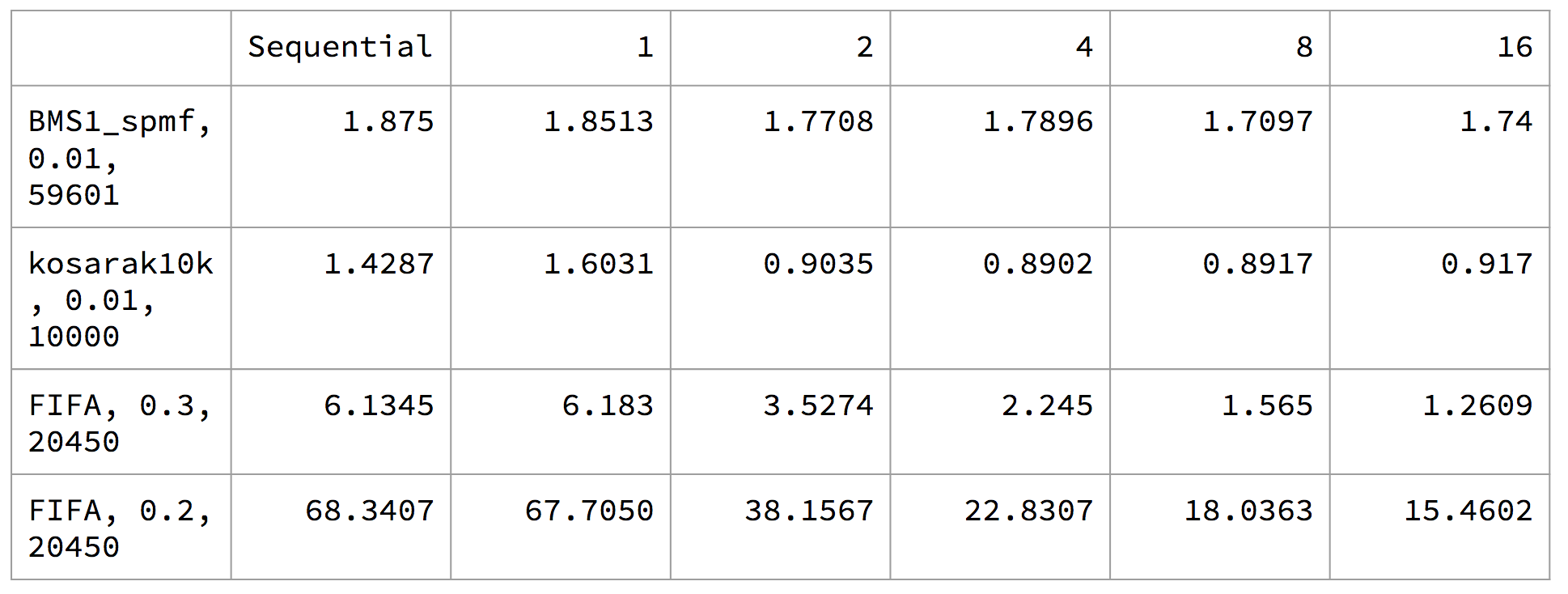
To measure performance, we compared the speedup between the baseline sequential algorithms and the parallelized algorithms we wrote by looking at wall-clock time it takes for the algorithms to output all of the frequent sequential patterns. We used four tests with three databases from here: BMS1_spmf (59601 sequences), kosarak10k (10000 sequences), and FIFA (20450 sequences). We used minsup=0.01 for BMS1_spmf and kosarak10k, and minsup=0.2 and 0.3 for FIFA. We chose these values to ensure we get a reasonable number of frequent sequential patterns considering the time limit we have on the GHC machines.

The execution time for PrefixSpan:

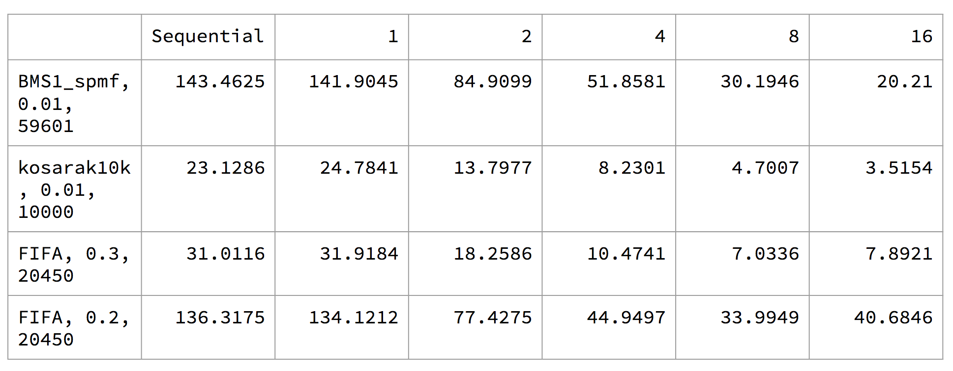
The execution time for GSP:

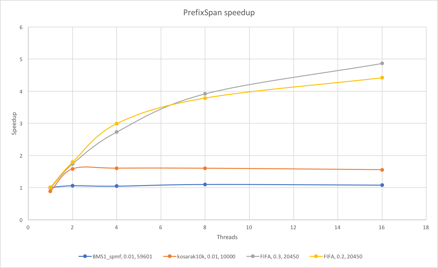
The speedup plot for PrefixSpan compared to the baseline sequential CPU implementation:

The speedup plot for GSP compared to the baseline sequential CPU implementation:

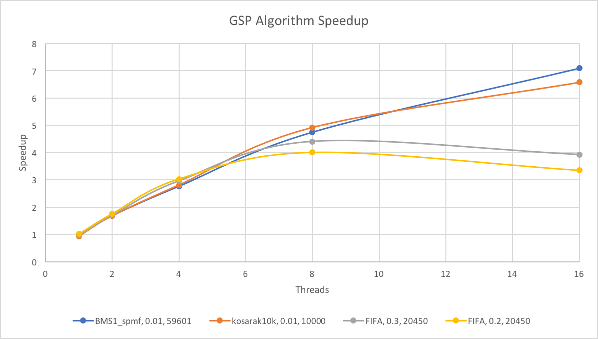
We note that there are two distinct groups for the tests: the two tests for FIFA vs BMS1_spmf and kosarak10k. For the GSP algorithm, we see that BMS1_spmf and kosarak10k exibits near linear speedup, but the FIFA tests plateaued at around 8 threads. We speculate that this may be due to workload imbalance due to candidate generation, as the parallelism we have across frequent k-1 sequences have divergence, and not every frequent k-1 sequence will generate the same number of candidates.

For the PrefixSpan algorithm, we see that for BMS1_spmf and kosarak10k plateaued at a very few number of threads. We suspect that this is due to the overhead of task creation. For these two datasets, the number of frequent patterns is relatively low, with most having much fewer supports than those from FIFA dataset. This means that the projected databases for these frequent patterns is much smaller, and the computation cannot take advantage of parallelism very well. Rather, the task overhead becomes significant. On the other hand, for FIFA dataset, the frequent patterns are well supported, suggesting that the projected databases are much larger to exploit the data parallelism as well as the task parallelism defined in this algorithm.

While my implementations showed good results for the GHC machines, I wish I was able to test on bigger inputs to mimic real life situations. In particular, I think data mining algorithms can also benefit from parallelism across machines, especially when the dataset is too large to fit on one disk. Because I was using GHC machines, I was not able to run datasets too large as that would take away resources from other people using the machines.

References

[1] Han, Jiawei, et al. "Prefixspan: Mining sequential patterns efficiently by prefix-projected pattern growth." proceedings of the 17th international conference on data engineering. 2001.

[2] Srikant, Ramakrishnan, and Rakesh Agrawal. "Mining sequential patterns: Generalizations and performance improvements." Advances in Database Technology—EDBT'96 (1996): 1-17.